An introduction to FLINT modules

info
This page is incomplete and we would love your help. Edit this page and add anything that would be helpful to others.
FLINT is a tool designed to support better land management and help reduce greenhouse gas (GHG) emissions worldwide. The tool uses modules to simulate different environments and processes related to carbon transfer.
A module is a self-contained set of operations that describe the ecological processes driving carbon changes in a landscape across a specified period. For example, the empirical forest growth module contains all the operations needed to simulate biomass accumulation.
All modules are compatible with the develop branch of FLINT, and any actively maintained branches will work with the most recent version. It is strongly recommended always to use the latest version of FLINT. The FLINT Application Programming Interface (API) has evolved so that some modules might be outdated.
Modules come in three different tiers according to the amount of information they need and their degree of analytical complexity. Three tiers are described for categorizing both emissions factors and activity data. Tier 1 is the most basic, frequently utilizing IPCC-recommended country-level defaults. While tiers 2 and 3 are more advanced.
Prerequisites
Before learning more about modules, you should take the time to familiarize yourself with FLINT and how it works. For more information, see GitHub - FLINT repository.
Contents
- How do modules work?
- Empirical forest growth module
- Hybrid forest growth module
- Turnover module
- Decomposition module
- RothC soil carbon module
- Chapman Richards module
- GCBM module
- WOFOST crop growth module
- Frequently asked questions
How do modules work?
Modules are responsible for managing "state variables" and "carbon pools".
- State variables are variables that can represent characteristics of the environment such as tree height or age.
- Carbon pools represent the location of carbon within an environment. Such as in trees, underground or in the atmosphere.
Each module must ingest data such as climate data or information about environmental disturbances to calculate changes to state variables and the amounts of carbon in each of its carbon pools as the simulation progresses.
At the end of a simulation, modules output the updated values for state variables. The output for carbon pools is in the form of an array (sparse matrix). The array includes information about the source pool, the sink pool, and the amount of flux. The module output is shared with the unit controller within FLINT.
Modules run over "simulation units". A simulation unit can represent a spatial area, such as a forest, or an emissions source, such as livestock. When the simulation unit refers to a geographical area, it is known as a "land unit". FLINT is responsible for managing the processing of simulation units over time.
Pools
A pool is a reservoir within which something can be stored and released. For example, a carbon pool is a reservoir from which carbon can be stored (sequestered and maintained) or emitted, such as debris. Within FLINT, each pool has attributed a value such as tonnes of carbon, and at each time step, the FLINT can move stores from one pool to another using an operation. Here is an example of pools in a FLINT simulation.
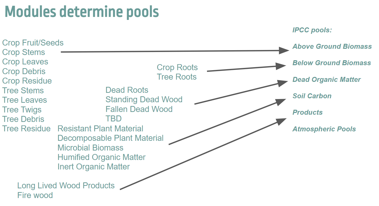 |
|---|
| Diagram depicting how modules determine pools in FLINT. |
Operations
An operation is a process within FLINT that moves carbon stock between pools. Operations can reflect ongoing natural processes, such as growth, or specific events, whether natural or human-induced. Operations allow FLINT to track changes in carbon stock through time, including fluxes into and out of pools. For example, a harvest operation moves plant material to products and debris pools, whereas a wildfire operation moves plant material to debris and atmosphere pools.
Events
Events are operations that occur intermittently (rather than for every step in a simulation), resulting in the movement of carbon from one pool to another. Events include natural and anthropogenic events, including fire, harvesting, ploughing, and fertiliser application. These are coded for the FLINT as a module. Here is the relationship between Pools and Operations/Events.
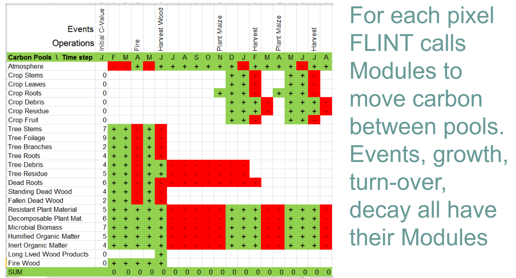 |
|---|
| Diagram depicting how FLINT calls modules to move carbon between pools. |
Temporal distribution
The temporal scale in FLINT is referred to as time steps. Time-steps are lengths of time over which operations are reported. At the end of a time-step, carbon can be moved from one pool to another.
The standard time step in FLINT is one month. However, it can be varied by the user. One month is the recommended time step for modelling carbon.
Synchronized events
In some circumstances, simulated modules for a particular Simulation Unit are dependent on other Simulation Units. That is, the Simulation Units are interdependent. In these situations, it is necessary for a process that synchronizes across the related Simulation Units, which is known as synchronized events. The Synchronized Server in FLINT manages Synchronized events.
Mass balance
The carbon cycle is based on the transfer of carbon molecules from one pool to another, where the molecules are not created, nor are they destroyed. As such, all outputs must be equal to the inputs. The system must be in balance. This is referred to as mass balance.
Existing FLINT modules
Empirical Forest Growth Module
The empirical Forest growth module includes all operations required to simulate biomass accumulation. It simulates the growth in carbon stock within a forest over time. This module is included within FLINT and is also used by the Chapman Richards Module. Biomass refers to the mass of living organisms, including plants, animals and microorganisms. Biomass accumulation is the net change in standing Biomass from one time to another (g/m^2).
The module runs at a monthly step interval. The module's behaviour is based on yield tables representing monthly growth increments for a forest type. The data for the yield tables comes from research and experimentation and is called empirical data, thus giving the name of this module, the empirical forest growth module. It's important to note that the yield tables only include above-ground biomass. If you want to calculate the *below-ground Biomass, you should use the hybrid forest growth module.
Inputs:
- Time Step (Monthly)
- Species
- Age
- Region
- Forest type
- Pool 1: Stemwood
- Pool 2: Bark
- Pool 3: Leaves
- Pool 4: Coarse Root
- Pool 5: Fine Roots
- Rainfall in that region
- Minimum and Maximum Temperature
- Vapour Pressure Deficit
- Soil Water Holding Capacity
Outputs:
- Calculated above-ground and below-ground Biomass.
Hybrid Forest Growth Module
The Hybrid Forest Growth Module calculates the biomass above and below the ground. The module simulates physiological responses to environmental conditions to help derive relationships that we can use to predict tree growth. The module contains a series of equations used to calculate the amounts of biomass in the environment.
The Hybrid Forest Growth module represents a 3-PG model (Physiological Principles in Predicting Growth). 3-PG models require more detailed data than is typically needed in empirical growth models. 3-PG models are better than the empirical models as we can use them with any landscape as long as all the required data is provided.
In forestgrowthmodule.cpp, the equation used is:
double ForestGrowthModule::calculate_above_ground_biomass(double age, double max, double k, double m) {
    return max * pow(1 - exp(-k * age), 1 / (1 - m));
}
Turnover Module
Turnover is the movement of carbon from a living carbon pool to a dead carbon pool. It is due to the natural living process of plant components. For example, a deciduous forest will have near 100% turnover of leaves across a year or an annual turnover rate of 99%. The turnover rates will vary with vegetation types and the plant components. For example, A tree stem may have zero (0) annual turnover, while the leaves have one (1).
To determine the volume of turnover through time, a calculation similar to the one below is carried out:
Turnover= 1 - (1 - turnover_rate) ^ time
Within FLINT, the maximum decay rate is 0.99 999 999 998, and the minimum decay rate is 0.000001. These limits are in place to ensure there are no invalid calculations occurring in the system.
Decomposition Module
Decomposition represents heterotrophic respiration of litter and soil organic matter. The process of modelling decomposition is similar to turnover in plant material, where a proportion of biomass in litter and soil organic matter decays through time. The rates of this vary with location based on the environmental conditions.
RothC Soil Carbon Module
RothC is a module used to simulate soil carbon turnover in non-waterlogged soils under different vegetation types. It is based on the decomposition of organic matter related to mean temperature and moisture and the proportion of resistant and decomposable organic material. It runs on a monthly time step interval.
Input data for the RothC module is readily available. There is considerable overlap between hybrid growth modules and WOFOST modules. For a detailed explanation and better understanding, see Ver de Terre production - RothC guide.
Inputs:
- Time Step (Monthly).
- Pool 1: Input of plant residue.
- Pool 2: Input of farmyard manure.
- Pool 3: Total organic carbon.
- Pool 4: Microbial biomass carbon.
- Rainfall.
- Open pan evaporation.
- Mean air temperature.
- Clay content of soil.
- Decomposability of incoming plant material.
- Soil cover.
- Depth of soil layer sampled.
Output:
- Total Organic Carbon.
- Microbial Biomass Carbon.
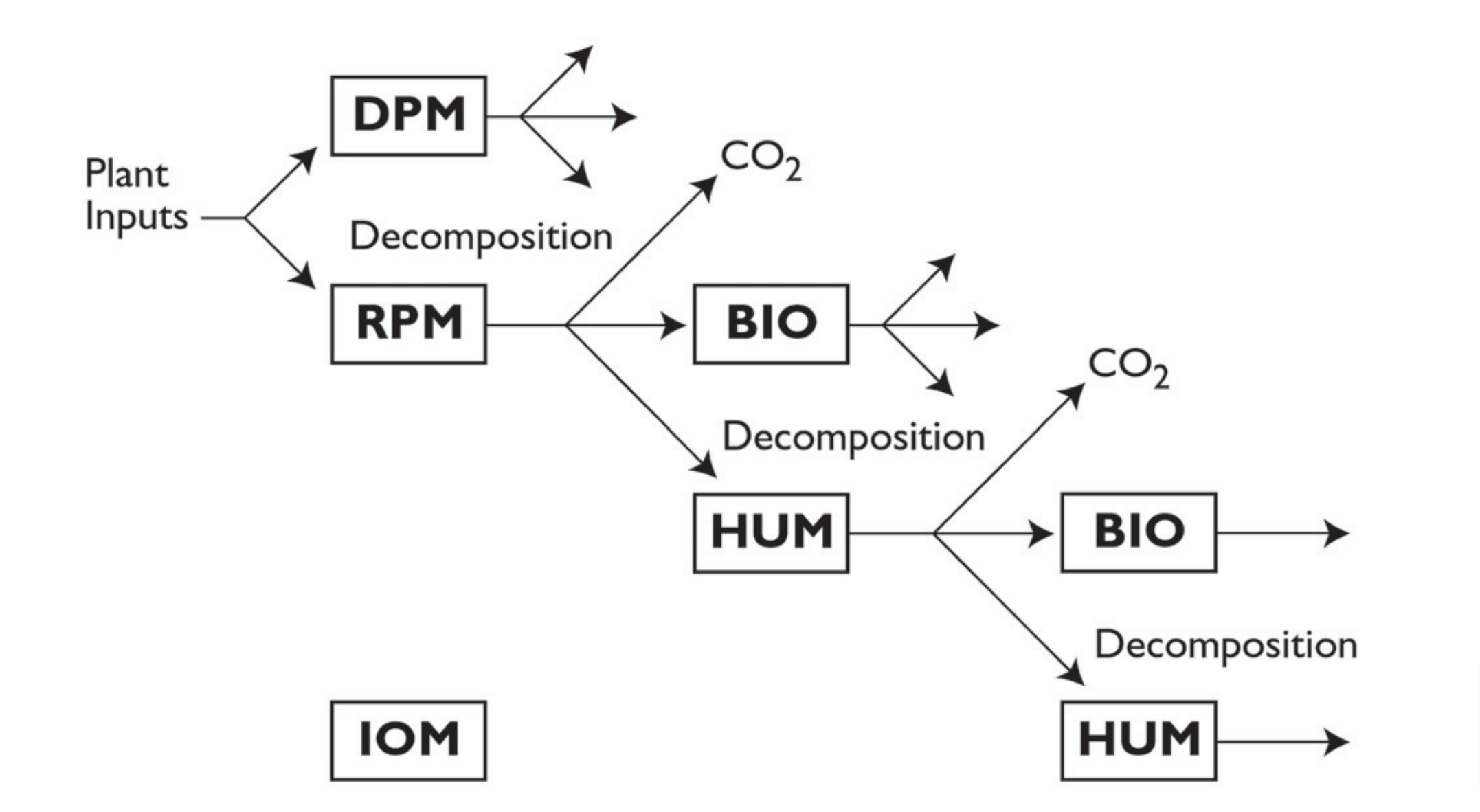 |
|---|
| Pictorial representation of RothC Module. |
Chapman Richards Module
The Chapman Richards module is a tier 3 module. It is used to estimate greenhouse gas emissions and removals due to changes in biomass carbon for forests using the Chapman Richards equation. We can calculate above-ground and below-ground biomass using this module.
AGC = * [ 1 - e ^ { -k *Age } ] ^ { ( 1 / (1-m) }
- AGC: Above-ground stand carbon (Tonnes carbon per hectare).
- Max: Asymptote – maximum peak carbon yield (Tonnes carbon per hectare).
- k: Parameter used in modelling tree growth (dimensionless).
- Age: Age of the forest (years).
- m: Parameter used in modelling tree growth (dimensionless).
This module estimates above-ground biomass based on the age of forests. Below-ground biomass is calculated as a ratio of above-ground biomass. This equation is also used within the Forest Growth module. A separate repository for the Chapman Richards module is available. It works on a monthly time step interval.
Input
- Time Step (Monthly)
- Dead Organic Matter
- Soil organic matter
- Pool 1 : Non-CO2 gases (The selection of carbon pools or non-CO2 gases for estimation will depend on the significance of the pool and tier selected for each land-use category)
- Forest Age
- Forest Type
- Forest Cover
- Soil Carbon
- Spatial Location of Forest
Output
- Above-ground biomass
- Below-ground biomass
GCBM Module
The Generic Carbon Budget Model (GCBM) is a set of science modules developed by the Canadian Forest Service (CFS) to run with FLINT.
These are the same science modules used in the first generation tool (CBM-CFS3). Since the science and processes behind both tools are very similar, it is relatively easy to transition from CBM-CFS3 to GCBM.
The CBM-CFS3 is widely used throughout Canada and globally. Its use is supported by the Canadian Forest Service of Natural Resources Canada.
The next generation GCBM is currently used by the CFS with several partner organizations to advance the science of forest carbon estimation and support policy analyses such as assessing mitigation options in the forest sector.
In GCBM, forest inventory and disturbance events are spatially explicit. The location of disturbances is explicit in spatial layers. The GCBM Module can simulate large landscapes easily.
 |
|---|
| Diagram depicting the high-level overview of GCBM. |
The module works at an annual Time step interval. There is a special repository for the GCBM Module.
GCBM sub-modules
There are a large number of modules within the GCBM, some of which are optional depending on your simulation requirements. We have only included a short summary of these modules.
Canadian Model for Peatlands (CaMP)
The Canadian Model for Peatlands (CaMP) is a module for Greenhouse Gas (GHG) emissions. The CaMP was designed as a module for the spatially-explicit GCBM. The CaMP is a site to a national-level peatland carbon model developed to estimate GHG emissions across a range of peatland types in Canada.
Different events are triggered based on the land type found during the simulation. For example, if the land type is peatland, this triggers a peatland disturbance event. Otherwise, it triggers a regular CBM disturbance event.
Decay Module
This module calculates the annual decay and turnover of a set of dead organic matter pools present in the GCBM. The data requirements for the decay module are:
- A table named "decay_parameters", with one set of decay parameters for each of the enumerated Dead Organic Matter (DOM) pools in the DOMPool.
- Scalar "mean_annual_temperature". This is the mean annual temperature of the environment.
- Scalar "SlowMixingRate". This is the amount that has moved from slow above-ground to slow below-ground annually.
Moss Decay Module
This module is used for moss related computing. This module determines whether the moss pool is decaying. Different decay rates can be applied to different pools.
Moss Disturbance Module
This module responds to the fire disturbance events in GCBM. This module is responsible for transferring carbon content from moss pools to the atmospheric emission pool. It gets the input data from the variable: moss_fire_parameters.
Moss Growth Module
This module is responsible for the growth of moss pools.
Moss Turnover Module
This module is responsible for the turnover of moss pools. The movement between the moss live pool and the moss past pool. This module calculates the movement between the moss live and pools, in response to the transfer rates assocated with different simulation events.
Peatland after GCBM Module
This module is triggered after GCBM simulation on a land unit, and prepares the land unit to simulate the peatland simulation. It transfers carbon from some GCBM pools to the peatland pools. It is called after finishing the regular GCBM simulation.
Peatland Decay Module
This module is responsible for peatland decay. It uses the variables: peatland_decay_parameters and peatland_turnover_parameters. It also uses various parameters like: mean annual temperature, annual water table depth, total initial carbon.
Peatland Disturbance Module
This module responds to the historical and last disturbance events in the GCBM spinup. It alters the water table depth according to the disturbance type.
Peatland Growth Module
This module gets the data from the variables: peatland_growth_parameters, peatland_turnover_parameters and peatland_growth_curve. It simulates the various growth cycles, growth curves and also sets the component value for the pools. For example: woody layer, moss layer and many more.
Tree Growth Module
This module deals with the small trees growth curve ID like black spruce. There is a peatland pre-defined forest growth curve of black spruce. It takes the current eco boundary variable name and then checks if it was changed or just set. As output, it updates the small tree growth curve parameter. It calculates the biomass transfer between various tree pools like stem wood, coarse root, with the help of the age of the small tree.
Stand Maturity Module
This module creates the stand growth curve. It gets the standard growth curve ID associated with the pixel, processes it and converts the yield volume to carbon curves.
Tree Yield Table Module
A yield table is a table which indicates the volume of wood per unit area of forest that is expected to be at different ages compared to other trees.
This module creates the yield tables for multiple hardwood and softwood species components depending upon the tree's age, species type and species ID of the tree.
It also summarises the total volume of the species growth curve and creates a yield table for a specific type with the transform result yield data.
Yield Table Growth Module
This module creates and updates yield tables for different land types like peatland and moss and transfers content between various biomass pools. It requires the growth yield curve to work, which it retrieves from the stand growth curve factory file. It also performs turnover and decay of different pools in one step.
The Turnover module and the Decomposition module are also used as a pre-requisite for the GCBM.
Input
There are no specific inputs to the GCBM module. It contains several modules which have multiple inputs and they all interact with each other to produce the output of GCBM in the form of maps and tables.
Output
GCBM gives us the estimate of carbon flux generated, above-ground biomass etc. There is a special repository to visualize the output generated by GCBM called Taswira.
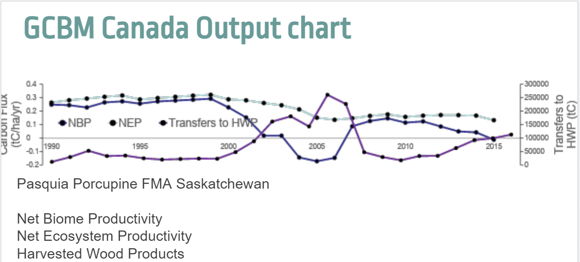 |
|---|
| Diagram depicting how the GCBM output is displayed on a chart. |
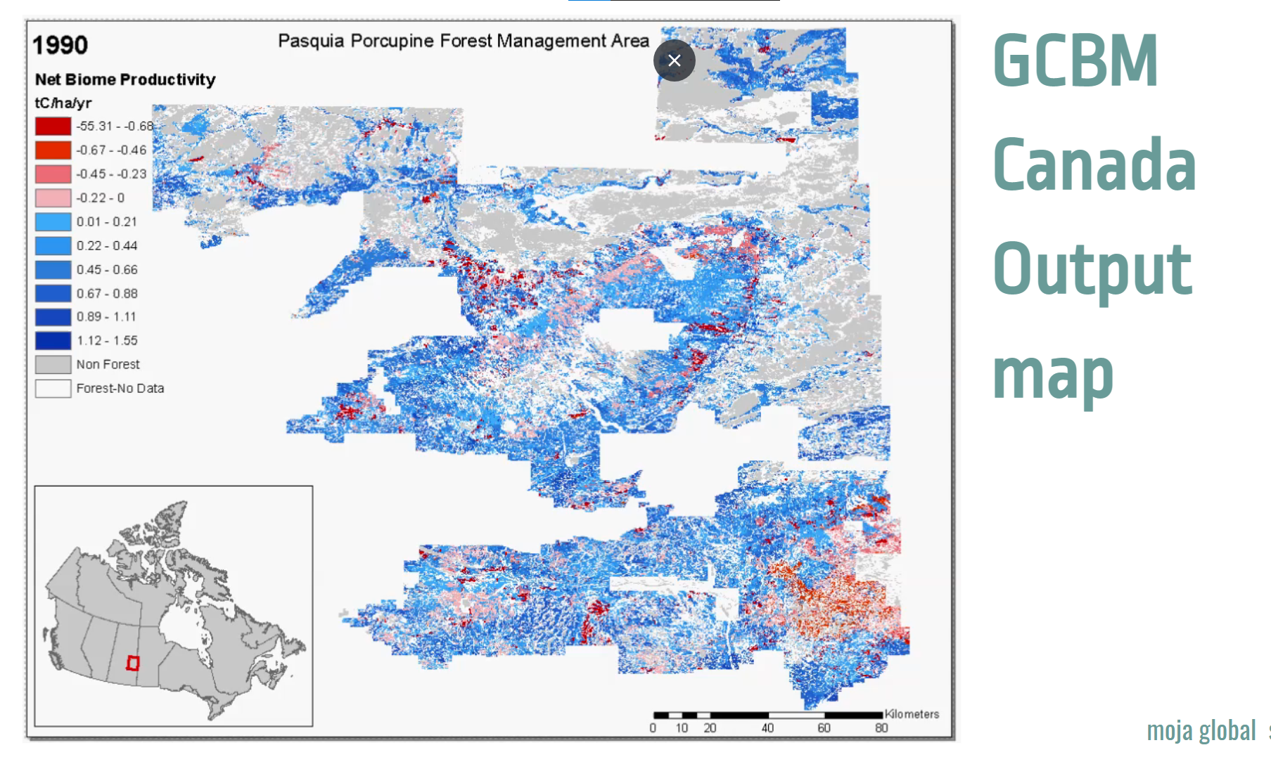 |
|---|
| Diagram depicting how the GCBM output is displayed on a map. |
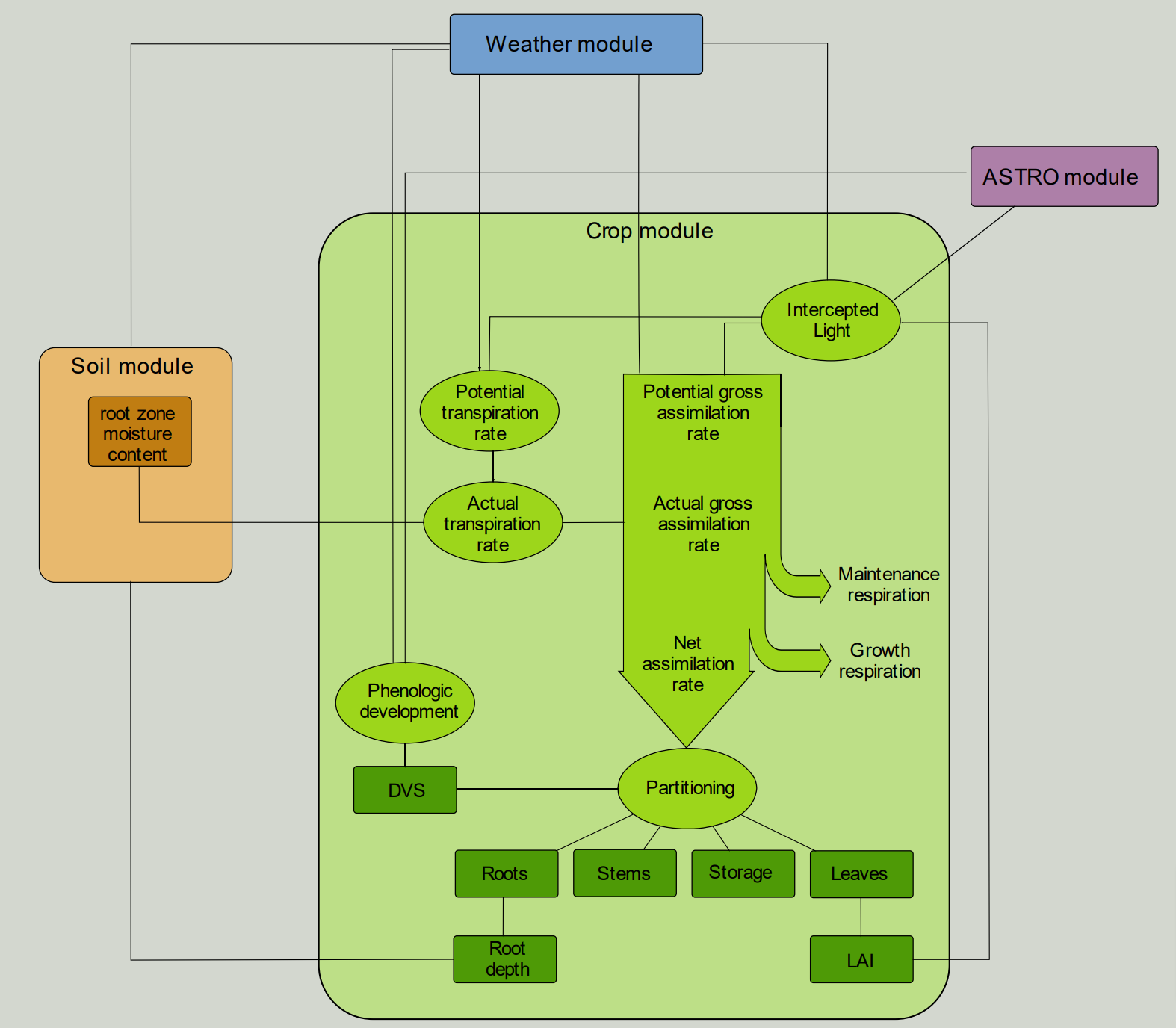
Wofost Crop Growth Module
WOFOST (WOrld FOod STudies) is a mechanistic module that simulates crop growth based on photosynthesis, respiration and the prevailing environmental conditions. It is similar to the hybrid forest growth module.
It is similar to the DayCent. This module runs on a Daily time step and allows users to model the potential production, attainable production and actual production for a given site (region). The simulation runs from sowing to maturity and is based on the response of the crop to weather (all production levels) and soil moisture conditions.
Inputs:
- Time step (Daily)
- Crop Type
- Pool 1: stem
- Pool 2: Leaves
- Pool 3: Storage Organs
- Pool 4: Roots
- Maximum and Minimum Temperature
- Global Radiation
Outputs:
- It calculates how much carbon moves between pools.
 |
|---|
| Pictorial representation of WOFOST Module. |
Frequently asked questions
Do modules need a specific version to run?
The modules work with the
developbranch of the FLINT. We recommend you use the latest version of FLINT available.Why are modules important?
Without modules, FLINT can't produce any output. Each user has different data, policies and reporting needs. Based on these needs, users select the appropriate modules and data to use with FLINT.
Where can I learn more about modules?
To deepen your understanding of modules, you have to understand how a module works, what the different operations are in FLINT, and how it is being managed and developed. The metric and carbon calculation modules docs contain more advanced information.
Can I implement a module from scratch?
Yes, you can. Here's an example of a custom made module: Agricultural soil module. This project involves specifically implementing the agricultural soils model used to estimate non-CO2 GHG emissions from agricultural practices. You can visit the module development docs to learn how to implement a single, simple module from scratch.
How do modules interact with each other?
Different Modules are configured through the local domain controller and sequencer which decides the flow of modules. Below is a sequence diagram to help you visualize this flow.
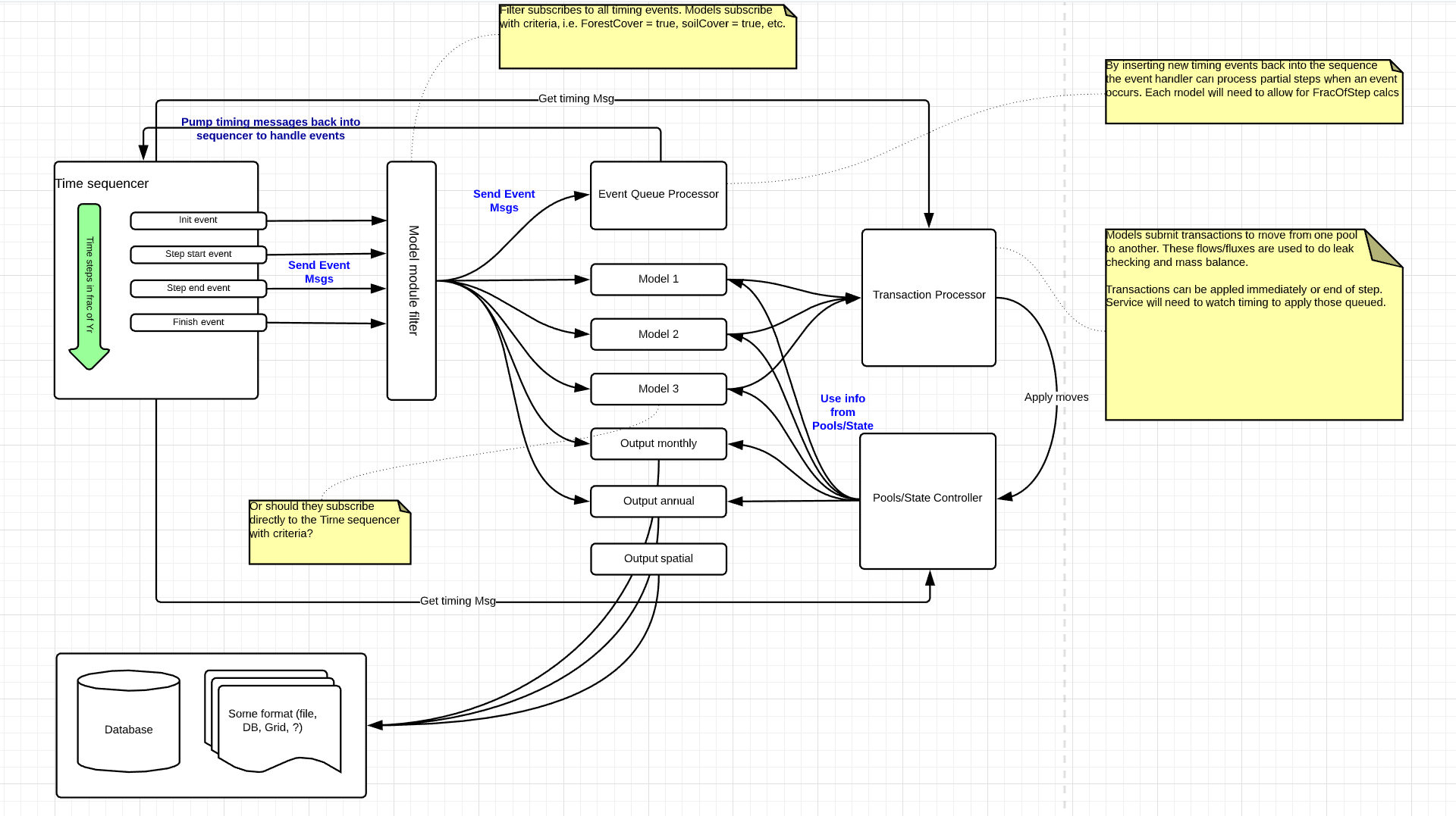
Diagram depicting the control flow diagram of how FLINT modules interact with each other. How can I implement a module from scratch?
If you would like to implement a new module, please reach out on
#modules-and-gbcmon Slack.